Posts Tagged ‘PivotPoint’

New versions of PivotPoint and TeamTime replace Adobe Flash based charts with HTML5/JavaScript

Date:June 4th, 2019 Author: Tags: , ,
Category: PivotPoint Web Part, SharePoint TeamTime Comments:0 ;

New versions of PivotPoint (v4.1.2) and TeamTime (v4.1) are available that replace Adobe Flash based charts with HTML5/JavaScript charts using the ChartJS library.

PivotPoint

Adobe Flash is set to be discontinued at the end of 2020 and major browsers like Chrome already require permission to enable Flash each time the browser is restarted in an effort to speed up the move away from Flash to alternative technologies.

The JavaScript charts will be used automatically on SharePoint 2013 and above (but you can switch back to Flash if you wish).

Internet Explorer (even IE11) do not support HTML5 when running with SharePoint 2007 and 2010 so they will continue to use Flash on these old versions of SharePoint. If you are using other browsers like Chrome or Firefox with older versions of SharePoint you can override this to force it to use JavaScript charts on these older versions of SharePoint too.

You can upgrade by simply installing over the top – your settings will be saved. (As with all SharePoint installations please do this out of hours)

NOTE – you may need a new license key issuing if you currently have an older major version (e.g. anyting less than v4.x). This is included if you have an active Premium Support and Maintenance agreement in place. If you are unsure please check with us!

Google Chrome v43+ incompatibility – new version of Planner, PivotPoint and TeamTime available

Date:June 1st, 2015 Author: Tags: , , , , ,
Category: PivotPoint Web Part, SharePoint Planner, SharePoint TeamTime Comments:0 ;

New versions of Planner, PivotPoint and TeamTime are available that correct an incompatibility with Google Chrome v43+.

This incompatibility can cause the web part to be hidden when using the web part configuration toolpane (edit web part).

As Google Chrome is automatically updated it’s important that any customers who use Chrome update to the latest version.

You can download the latest trial version and upgrade by installing over the top – your existing settings will be saved and the License Key picked up to activate the full version.

Add Highlighting & Conditional Formatting to PivotPoint tables

Date:March 12th, 2014 Author: Tags: , , , , ,
Category: PivotPoint Web Part, SharePoint Ideas Comments:1 ;

Our PivotPoint web part for SharePoint allows you to summarise data from your SharePoint lists in a similar way to Excel’s Pivot Tables and Charts.

A few users have asked how you can add highlighting or conditional formatting to the Pivot Tables – to do things like highlighting the High Risk column, or any cell above a certain value.

We have a Highlighter app that allows you to do this on normal Lists but it doesn’t work with PivotPoint so I thought I would put together some examples of how you can do this using every SharePoint hackers favourite tools – JavaScript and jQuery.

You will need some experience with programming and/or JavaScript to be able to modify these examples to do what you want but there are lots of comments in the code to help.

If you’re looking for an easy way to add conditional formatting/ highlighting for SharePoint Lists then check out Highlighter.

So lets get started. The files you need for the article can be found in a zip file here. Inside you will see a test .html page that can be used just to experiment with the javascript and a .js.txt file that contains the javascript to use on your site.

Adding JavaScript to a page

The first thing we need to know is how to add JavaScript to a page. Read up about that and come back!

In SharePoint 2013 you can add a Script Editor web part (under Media and Content). This blog post walks you through.

For SharePoint 2010 and 2007 you have to use the Content Editor web part (CEWP)

You could use the Source View of the CEWP and put the JavaScript directly into it, but you could also staple your tongue to a door and it will probably be less painful!

A much better way is to save the script as a .txt file in a document library and then include the file on the page with the Content Editors “Content Link” feature. Christophe walks you through this method here.

jQuery or not?

The examples given here use jQuery – a great addition to JavaScript that simplifies many common tasks.

You could adapt these ideas to run without jQuery if you like – but you’re on your own with that!

You can see the reference to jQuery on the first line of the example scripts.

One thing you should determine is

a)      Has jQuery already been added to all your SharePoint pages (by an administrator adding them into a custom master page)? If so then you should remove the jQuery reference from these examples as there is no point in including it twice.

b)      These jQuery files are loaded from Googles CDN servers. If you don’t have external internet access you will have to copy jQuery to some other location (such as a document library).

Show me the examples already!

Download and unpack these zip files – inside you will see

.htm files that you can experiment with.

Open them in a browser to see what they look like. Open them in a text editor like Notepad to change how they look and then re-load in the browser (F5).

.js.txt files that you can use in SharePoint.

Use a text editor to copy the changes you’ve made in the example .htm file in and then add them to the page that you have PivotPoint on using any of the methods in “Adding JavaScript to a page”.

The two examples are :-

Highlighting PivotPoint cells based on the value

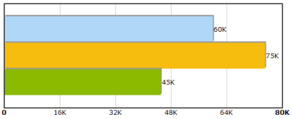
The first example we’re going to look at is to highlight different cells depending on the value that’s in them.

For our example –

  • If it’s less than or equal to 160 then we want the text in red
  • If it’s more than or equal to 180 then it should have a background in yellow.

The result should be a web part like this.

highlight-by-cell-value

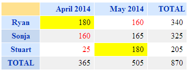
There are plenty of comments in the JavaScript source code but basically what it’s doing Is looping through each cell in the PivotTable, checking what value It is and applying a CSS style.

See the source of highlight-by-cell-value.html and highlight-by-cell-value.js.txt in the ZIP file


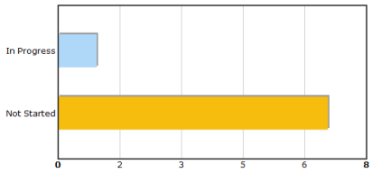
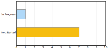
Highlighting PivotPoint based on the row and column

In this example we’re looking to highlight a cell based on what Row and Column it appears in.

E.g. in this risk matrix we want to highlight the “High Risk” and “Frequent Probability” in red.

risk-matrix

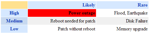
There are two ways to do this in the javascript example given.

The first is to highlight based on the position, e.g.

highlightCellByIndex(0,0,'background','red');

Will highlight the cell in column 0, row 0 by setting the background red. (Yes sorry, the rows and columns start from number 0!).

But – if the layout of your table changes in future (e.g. someone adds a “Super Extra High Risk”) column) then everything will move and this will be in the wrong place.

In that case the better way is to highlight by the value of the Column and Row headers – e.g.

highlightCell("Rare","Low", 'background','red');

See the source of highlight-by-column-and-row.html and highlight-by-column-and-row.js in the ZIP file

Tips –

  • When making changes to the javascript do a small amount at a time, then you will know where to start if this doesn’t work!
  • You’re not just limited to setting colours, you can also add in any other effect possible in CSS.
  • Use the developer toolbar (F12 in IE and Chrome) if you have an error – this tool will enable you to track it down, but how to use it is beyond the scope of what we can show here!
.css('font-weight','bold');
.css('font-size','200%');
.css('border','1px solid red');
  • You can also add images (e.g. flags)
.append("<img src='some-url-to-an–icon.gif'>");


Disclaimer – these technique is provided as is and free of charge to get you started. You will need some experience of JavaScript or programming and the browser developer tools to modify these to do exactly what you want. Whilst we can’t provide technical support for this we will endeavour to help customers with active Premium Support and Maintenance contracts in place for PivotPoint.


New version of PivotPoint – chart axis controls

Date:June 13th, 2013 Author: Tags: , ,
Category: PivotPoint Web Part Comments:0 ;

A new version of our PivotPoint web part for SharePoint is available – v 2.4.4

This new version adds options for manually controlling the scale and layout of the axis in charts.

Auto Scale

If you show values on the graph the Auto Scale option will scale large numbers to improve the display. For example 10,500 will be shown as 10.5K and 50,000,000 will be shown as 50M

pivotpoint-auto-scale

Axis Maximum & Number of Division Lines

Normally the maximum value on the axis and how many division lines are used is set automatically based on the data you’re charting. However with some settings – particularly small numbers it doesn’t always get it right. For example :-

pivotpoint-auto-axis

You can now manually specify these settings, in this example the axis is set from 0 to 10 with 10 division lines giving divisions at every exactly 1 intervals for a much better looking chart.

pivotpoint-manual-axis

More details are in the online manual.

You can download and upgrade to the latest version without losing any settings.

.

PivotPoint web part is now compatible with SharePoint 2013

Date:January 17th, 2013 Author: Tags: ,
Category: General, PivotPoint Web Part Comments:0 ;

Our PivotPoint web part is now compatible with SharePoint 2013 as of version 2.4.0.

You can download and install the latest version here.

If upgrading from SharePoint 2010 to SharePoint 2013 simply perform the upgrade then install the latest version – your old settings and license key will be picked up.

This page will be updated as our other web parts are made SharePoint 2013 compatible

PivotPoint web part

New version of PivotPoint web part for SharePoint – v2.2.3

Date:May 15th, 2012 Author: Tags: , , ,
Category: General, PivotPoint Web Part Comments:0 ;

A new version of our PivotPoint web part for SharePoint (v2.2.3) is ready.

This new version improves performance for large lists, corrects bugs when you have angled brackets (“<” and “>”) in your row or columns, adds support for site column lookups and a 2 new features.

Sort by Title or Total

The new version of PivotPoint allows you to sort by both the Title and Total rows, either ascending or descending.

Title and Total cells

For example, instead of sorting alphabetically by product you can sort by their total sales – showing your best performing products at the top of the table or left of the chart.

PivotPoint showing all columns

More details are in the online manual.

Show Top N

In combination with sorting by the Total you can choose to show the Top N columns or rows.

For example given the following data the vast majority of revenue comes from 2 products (Bottle-o-matic and Can-o-Matic) and we have a ‘Long Tail’ of other products.

We can choose to only display the top 2 columns (products) and optionally group all the other sales into “Other”

PivotPoint for SharePoint showing top 2 columns

 More details are in the online manual.

You can download and upgrade to the latest version without losing any settings.

Date Range filtering with the new version of FilterPoint, PivotPoint and Planner.

Date:December 13th, 2011 Author: Tags: , , ,
Category: Filter, FilterPoint Web Part, PivotPoint Web Part, SharePoint Planner, SharePoint webparts Comments:0 ;

FilterPoint has had the ability to send Date Filters but a common request has been Date Ranges – like showing everything this month, last year or between two arbitrary dates.

FilterPoint - Date Range Filtering

The good news is that we’ve added this in to FilterPoint as of version 1.2

The bad news is that this will only work with our other SharePoint products – Planner and PivotPoint – it won’t work with SharePoints built in List View web part (LVWP).

That’s disappointing!

Yes it is – it’s just a limitation of SharePoints filtering I am afraid, but all is not lost!

This page shows how you can do things like Month filtering using calculated columns and this blog article shows how you can setup “Current Month/Previous Month” views using nothing more than Calculated Columns and View filters.

Upgrading

As always you can upgrade without losing any settings by downloading and running the latest trial version and selecting “Upgrade” when prompted (don’t forget you need the a recent version of Planner (v2.6.9+) and PivotPoint (2.2.0+) to accept date range filters.

SharePoint Staff Vacation Planner Update – dealing with Public Holidays

Date:September 1st, 2011 Author: Tags: , , , ,
Category: PivotPoint Web Part, SharePoint Planner, SharePoint Reminder Comments:0 ;

Customers who use our SharePoint Staff Vacation Planner Toolkit often ask about the best way to deal with public holidays.  Public Holidays tend to affect the whole team.  So you want them clearly marked on your Vacation Planner dashboard, but you certainly don’t want to have to enter each public holiday for each team member as a separate event.  And you probably also don’t want to be firing off absence approval requests for each holiday either.

So here are our suggestions on the best way of handling Public Holidays within the SharePoint Staff Vacation Planner Toolkit.

First you need modify your list.  Go to list settings and open up your “Reason” field.  In addition to your existing reasons for absence add a new reason – Public Holiday.

Then open up the settings for your “Requested By” column and make sure you have “Allow Multiple Selections” checked.

Now you need to modify your Planner web part.

So, “Edit Shared Web Part” then, under your “Category”  picker, check the “split multiple selections box”.  This is key if you want to be able to create just one event for each public holiday but have it show up against each of your team members.

Now go down to the Planner Colors section of the Toolpart and update your color coding by column section to include an extra color code for your new Reason for absence that you created in your list – Public Holiday – I am going for a nice orange.

Now check your PivotPoint web part. For this to work you are going to need PivotPoint 2.1.4 or above.  Download it here if you don’t have it already (free to all PivotPoint v2 customers, or v1 customers with Premium Support). In the Toolpart make sure that in the “Split Multiple Values” dropdown you have chosen “Split Records”.  This will ensure that when we enter a 1 day public holiday for 4th of July, for example, 1 day gets entered against each team member in the pivot table.

Finally, before we start adding events, to ensure that we don’t accidentally fire off approval requests and notifications all over the place, access the Reminder web parts that you have set up and in the “Reminder Testing”  section at the bottom of the Toolpart enter your own email address so that any emails generated whilst you are adding the public holidays go to you.  This will be a better solution than simply switching the Reminders off as you work, as it will mean that if any “real” requests are submitted whilst you are working you will be able to redirect them, rather than them being lost.

Add a Public Holiday

So, from your Planner dashboard add a new item.  Let’s do 4th July. Set it up as an all day event.  Set yourself as “approved by”, you will need to approve the event before it will show up in people’s dashboards.  Now add your whole team to the “Requested By” field.  It’s easiest to do this using the Address Book.  Now ensure you have selected “Public Holiday” in your Reason field.  Approve the request.  Discard all the “Request approved” notifications that are redirected through to you.  And now you will see your public holiday, nicely marked against each of your team members.  Repeat as needed for all of your other public holidays, remove the redirect from your Reminder emails and then you can relax for another year!

I hope this helps you in using Vacation Planner.  If you have any questions or requests about the Vacation Planner we would love to hear them.

PivotPoint for SharePoint – New version Released v2.1.5

Date:August 31st, 2011 Author: Tags:
Category: General, PivotPoint Web Part Comments:0 ;

Only last month we launched PivotPoint v2, which added charting and drill down to this popular SharePoint tool.

Now we are releasing v2.1.5 which has some pretty nifty new features added as a result of your feedback on v2.

Axis Minimum

You pointed out that when looking at a chart, if all of your values are bunched between say 90 and 100, viewing them on an axis that runs from 1 to 100 doesn’t make things all that easy to read.

So the new Axis Minimum option lets you choose where your axis starts (in the example above this would be 90) making charts that much easier to read.

Split Multiple Values

In PivotPoint v2 we had disabled the option of using a multi-choice column. We felt that in most circumstances this simply didn’t make sense as an option within a Pivot Chart or Table.  But you disagreed, so we put the option to work with multi-choice fields back in and we think we have come up with a way of making it more usable.
So for example, take a simple task list – where as you can see the “Present Proposal” task is assigned to multiple people – Barry and Fred.

In your Pivot Table or chart you can choose to either treat your multi-choice record as a single record, effectively creating a new category in the Pivot Table, like this:

Or you can choose to split the multi-choice record between all the choice categories (in this case people) in it, like this:

If you choose to split multiple choice records between their multiple parts the full value of the record is allocated to each of its choices.

This brings PivotPoint in to line with the way that SharePoint Planner works, so will be especially useful for people who use dashboards with both Planner and PivotPoint deployed, and will also be very useful for our Vacation Planner users – watch this space for an update on how this is going to help you.

Allow Custom Field Types

Custom fields can cause all sorts of trouble, so previously we had simply outlawed them in PivotPoint in an effort to try and keep things simple.  However quite a few of you have said you wanted to be able to use custom fields, so we have now allowed you to enable this feature.

Be warned though, not all types of custom field will work correctly in PivotPoint (depending on their design) and we won’t be able to provide support on 3rd party custom fields.

Full information on all of these changes can be found in the PivotPoint manual.

Getting the Latest Version

PivotPoint v2.1.5 is free to download for anyone who has previously purchased PivotPoint v2, or PivotPoint v1 plus Premium Support.

Existing customers can download the latest version here.  The new version can be installed directly over the top of the old, and you will retain all of your existing web part settings.

For those of you using PivotPoint on a 30 day free trial, you can upgrade to the new version here, your trial will continue and you will retain any web parts you have set up already.

We hope you find these new features useful and we would love to hear your feedback on them, or any other aspects of PivotPoint v2.

Show Actual v Target Performance in SharePoint with PivotPoint web part.

Date:August 3rd, 2011 Author: Tags: , ,
Category: General Comments:0 ;

So we all like to know how we are doing – hitting our targets, meeting our KPI’s, staying within our budgets, running out of vacation days.

If you record things like this in SharePoint lists you would hope it would be easy enough to see how your actual performance compares to your targets, budgets or KPI’s.

Well for those of you who have Enterprise  and PerformancePoint it is possible – if not exactly a walk in the park –  but for the rest of us this can be a tricky task.   You need to find a way of bringing together 2 different sets of data:

  • Target or KPI – which is one item of data, which stays constant – no one likes a moving target do they?
  • and an “Actual” figure which is the sum of a number of list items – sales, purchases, leave bookings, whatever, and which will clearly change as list items are added and changed.

So if we were looking to compare Target and Actual sales for July, as in the chart above, the date would loook like this.  A list of sales items, which will grow as the month progresses, producing a changing Actual total,  and one Target item, which will stay the same throughout the month.

These two data sets would generally live in separate lists.  The way many KPI columns work is by getting you to manually enter – and manually update – your changing Actual total into your Target list.  Not great, as you never get to see how the situation is changing until you have done your manual update.

In a workaround for one of our PivotPoint customers we have turned this on method on its head – entering the static “Target” into the ~Actuals list (in this example the sales list) to allow you to produce a chart or table with our PivotPoint web part, which will show actuals vs targets and is updated as your actual data changes, without the need for manual intervention.

So here’s how.

Add a new column to your list.  Make it a choice column with the choices as “Actual” and “Target”.  Have it default to actual, as this is what the vast majority of items are going to be.

Then we simply enter a “Target” item for each category we want to compare.  So in this example I want to see actual vs target sales for each of my products. So I have entered a Target Sales item for each of my products for July.

As the month goes on my team will enter actual sales for July, which will (hopefully) start to stack up nicely against my target.

So to see how things are shaping up set up a PivotPoint, get it to watch the sales list, and in this case a “This Month” view of the sales list.  Display a Pivot Chart, in this case a column chart.

To see the actual sales vs target sales set it up like this:

  • Get your column data from the Actual/Target field.
  • Your Row data from the product field.
  • And your values from the Value field.

And you should end up with a nice column chart like the one above.

The best bit about this is that your chart will update as your list data changes.  So let’s say I get a really huge Planner order:

Woohoo – you can take that to the bank!

So, it’s not perfect, it’s a workaround, but some of you might find it useful.

Places you could use this would include:

  • Sales vs Target
  • Budget vs actual expenditure
  • Annual Vacation Allocation vs Vacation taken to date.

If you have any other ideas on where this might be useful we would love to hear them.